Abstract
Two observers granted independent, cloned access to the same bulk degree of freedom in a non-isometric holographic code can in principle disagree about its entropy. We quantify this disagreement in the AEHPV non-isometric framework with Harlow–Usatyuk–Zhao observer inclusion, and show it is governed by an entropy-replacement principle. Our main result (Theorem 1) is that the von Neumann entropy of an observer’s actual reduced state equals the Shannon entropy of its diagonal in the cloning basis, up to an error with – a full power of below the two-observer signal. For Haar-random bulk states this principle is established unconditionally, via an exact antisymmetric resolvent representation of together with a fourth-moment bound on the random-projection–induced perturbation. The replacement reduces the disagreement to a moment calculation of the bulk-marginal diagonal, which we carry out for two extreme bulk-state classes. For the Haar class we prove (unconditionally, Theorem 2) ; for random product bulk states we obtain, conditionally on the product-class replacement principle (Theorem 3), . The two exponents differ by exactly one power of , an instance of complexity-sensitive complementarity: the degree to which two cloned observers can disagree is set by the complexity class of the bulk state. All exponents and prefactors are exact asymptotics, supported by an extensive numerical program across the full HUZ+ pipeline.
§1. Introduction
1.1 Observer complementarity in non-isometric codes
In non-isometric holographic codes, the map from the effective (bulk) description to the fundamental (boundary) description is many-to-one: distinct bulk states can map to identical boundary data. This is the defining feature of the AEHPV construction, and it is what allows a black-hole interior to be encoded with far fewer fundamental degrees of freedom than the naive bulk Hilbert space would require. A consequence is that “an observer” is not a passive bystander: including an observer who measures a bulk degree of freedom changes the code, because the observer’s record must itself be encoded. The Harlow–Usatyuk–Zhao (HUZ) prescription makes this precise by cloning the measured degree of freedom into an observer register before the non-isometric map is applied.
When two such observers are included independently – each cloning the same bulk degree of freedom into its own register – the code now carries two records of the same information. Because the non-isometric map is not injective, the two observers’ reduced states need not agree, and in particular their von Neumann entropies need not agree. The size of this disagreement is a sharp, computable diagnostic of how much “room” the non-isometry leaves for observer-dependent descriptions.
1.2 The question
Concretely: let be a bulk state on , included for two observers and via HUZ cloning and mapped to the fundamental description by a fixed non-isometry built from a Haar-random isometry . Writing for the two observer-reduced states, we ask for the typical magnitude of
under the joint randomness of and (in two natural ensembles) the bulk state. How large is the disagreement, and what controls it?
1.3 Main results
The answer comes in two layers. The first is structural and is the technical core of the paper.
Theorem 1 (entropy-replacement principle, informal). The von Neumann entropy of an observer’s actual reduced state equals the Shannon entropy of its diagonal in the cloning basis, up to an error obeying
For the Haar bulk class this is a theorem, proved unconditionally in Appendix C; for the product class it is a conjecture, numerically supported but not proved. The proof for the Haar class is, we believe, of independent interest: it represents the antisymmetric entropy difference exactly through a resolvent integral, splits it into a linear piece (which reduces to the very bulk-marginal moment that controls the signal) and a nonlinear piece (controlled by a fourth moment of the random-projection–induced perturbation), and closes the fourth moment by a concentration estimate on the unitary group. The replacement error is suppressed relative to the signal by a full power of – which is exactly what is needed to make the entropy difference equal to the Shannon difference at leading order.
Given Theorem 1, the disagreement reduces to the variance of the Shannon entropy of the bulk-marginal diagonal, a classical random-matrix calculation. Carrying it out for two extreme bulk-state classes gives the second layer:
- Haar bulk states (maximal complexity), Theorem 2, unconditional: .
- Random product bulk states (minimal complexity), Theorem 3, conditional on the product-class form of Theorem 1: .
| Bulk class | Replacement (Theorem 1) status | Disagreement law |
|---|---|---|
| Haar | proved (Appendix C) | unconditional, |
| Product | conjectural / numerically supported | conditional, |
1.4 Physical interpretation: complexity-sensitive complementarity
The two exponents differ by exactly one power of . We read this as complexity-sensitive complementarity: the degree to which two cloned observers can disagree about a bulk degree of freedom is controlled by the complexity class of the bulk state. Highly scrambled (Haar) bulk states leave little room for disagreement – the disagreement falls off as – while simple (product) bulk states leave an order- more room, falling off only as . The non-isometry’s tolerance for observer-dependent descriptions is thus not a fixed property of the code but a function of what is encoded in it. Section 6 develops this reading and connects the exponent gap to the fluctuation structure of the bulk marginal.
1.5 Organization
Section 2 fixes the AEHPV/HUZ setup, the two-observer scenario, and the two bulk classes. Section 3 is the technical heart: it states and proves (modulo Appendix C) the entropy-replacement theorem, building it from the structural identity (Lemma 1) and the off-diagonal collapse, and verifies it numerically (Figure 2). Sections 4 and 5 derive the two scaling laws as consequences – the Haar law (Theorem 2, unconditional) first, then the product law (Theorem 3, conditional). Section 6 develops the complexity-sensitive reading of the exponent gap. Section 7 presents the numerical landscape (Table 1, Figures 1 and 5). Section 8 situates the results against EGH, HUZ, the Colorado rule, and the quantum-reference-frame literature. Appendix A records generalized EGH formulas; Appendix B documents reproducibility; Appendix C proves the entropy-replacement theorem for the Haar class – the resolvent representation, the linear and nonlinear bounds (Lemmas C.1–C.2), and the fourth-moment projector estimate (Lemmas C.3–C.5).
§2. Setup
This section fixes notation and conventions. We follow the AEHPV non-isometric-code framework [AEHPV 2207.06536], adapted to the two-observer scenario introduced by EGH 2507.06046 and HUZ 2501.02359. Readers familiar with these constructions may skip to §3.
2.1 Non-isometric maps and the AEHPV framework
The bulk effective theory and the fundamental (boundary) theory are two finite-dimensional Hilbert spaces connected by a linear map:
When , is non-isometric: there are bulk “null states” in the kernel of . Following AEHPV, we take to be the first rows of a Haar-random unitary on . This ensures exactly, while is a Haar-random rank- projector on . The non-isometry parameter is
Throughout this paper we fix .
2.2 Observer-included states via HUZ cloning
The HUZ 2501.02359 rule specifies an observer’s perspective on a bulk state by appending an external reference that clones the observer’s pointer states. In the single-observer case, the bulk factorizes as (observer and matter), and a reference register is added. The cloning isometry produces the HUZ map
Applied to any bulk state and normalized by post-selection, this produces a state on . The observer-accessible reduced state and its entropy are
2.3 The two-observer scenario
We consider the setup of EGH 2507.06046 and its natural refinement to two independent observers. The bulk effective space factorizes as
where and are two independent observer factors and is a matter register. Two auxiliary reference registers and of dimensions are introduced, and the two-observer HUZ map
is applied to the bulk state . The post-selection-normalized state is denoted .
The two observer-dependent entropies are
and similarly for . The central quantity of this paper is the Haar-averaged disagreement
where the expectation is taken over (Haar on ) and optionally over bulk states drawn from a specified class.
2.4 Bulk state classes
The theorems of this paper apply to two distinct bulk-state classes, each defining an ensemble over :
- Product class (P). Bulk states of the form , with each factor Haar-distributed on its respective Hilbert space. Such states have no bulk entanglement across the // partition; the -marginal is a rank-1 pure state.
- Haar class (H). Bulk states drawn uniformly from the unit sphere of (Haar measure on ). Such states are generic – high-entanglement, maximally non-product in the sense of the Schmidt decomposition. The marginals are close to maximally mixed with small Dirichlet-type fluctuations.
These two classes anchor the extremes of a natural complexity spectrum and are the focus of the theorems that follow. Intermediate classes (Schmidt-rank- bulk states) are a natural target for follow-up work, discussed in §6.5.
2.5 Parameters
Unless stated otherwise, all numerical work uses (so the setup is symmetric under observer exchange), , and (so ). The “scanned dimension” is . All averages refer to the joint measure over and bulk states; except where noted the two averages are independent.
§3. The entropy-replacement principle
This section establishes the technical heart of the paper: that the von Neumann entropy of an observer’s actual reduced state may be replaced, up to a provably subleading error, by the Shannon entropy of its diagonal. This entropy-replacement theorem (Theorem 1) is what licenses the entire reduction from a genuine quantum-information quantity to a classical moment calculation; the two scaling laws of §§4–5 are its consequences.
The proof has two ingredients, developed in turn. The first is a structural identity (Lemma 1): the Haar- expectation of the first-observer reduced state is, at leading order in , the diagonal in the basis of the bulk -marginal. This controls the mean. The second, and harder, ingredient controls the fluctuations: the replacement error has variance suppressed by a full power of relative to the two-observer signal. For the Haar class this is proved unconditionally (Appendix C); for the product class it remains a conjecture. The structural identity is established in §§3.2–3.3 and verified numerically in §3.4 (Figure 2); the entropy-replacement theorem is stated in §3.5, with its fluctuation bound proved in Appendix C.
3.1 Setup
Throughout we take to be an AEHPV non-isometric map with , fixed. Concretely, is the first rows of a Haar-random unitary on . The effective Hilbert space factorizes as
with the two observer factors and a matter register. Under the two-observer HUZ rule, both observers are cloned in their respective pointer bases, producing an auxiliary reference pair with . The post-, post-cloning normalized state is
Using index notation for the bulk-state components in the basis, and writing when factorizes across (we will treat the general case shortly), the unnormalized state is
The observer- reduced state is obtained by tracing out and , yielding
The norm is
3.2 The structural identity (Lemma 1): the Haar- expectation
The map is drawn from the Haar measure on the first rows of ; equivalently, is a uniformly random rank- orthogonal projector on . A basic moment identity gives
Applying (3.3) termwise to (3.1): the inner product enforced by the Haar first moment is , so the sum over (the index ) and the matter contraction collapse the off-diagonals already at first moment,
and
where is the bulk -marginal density matrix.
A subtlety: equations (3.4)–(3.5) are ratio-of-expectations statements, not the quantity of physical interest . These differ by fluctuations in . The following concentration estimate closes the gap.
Lemma 2 (Norm concentration). With of unit norm, , where is the Rényi-2 probability of the flat distribution over .
Sketch. From (3.2), is a weighted diagonal sum of entries. Using the joint second moment and the symmetry that is a uniformly random rank- projector (hence has joint diagonal distribution Dirichlet with fixed sum), one obtains the claimed variance bound directly. A detailed accounting gives for the state classes of interest.
Consequently concentrates around with relative fluctuation , and
This is the structural identity (Lemma 1): at first moment the observer register sees only the cloning-basis diagonal of the bulk marginal, not the full marginal.
3.3 Why the off-diagonals collapse
The collapse in (3.4)–(3.6) is a first-moment effect, not a variance effect. The single record held in labels the cloning index ; tracing out the other observer’s register together with the Haar first moment of contracts the two copies of the state at equal index and enforces . The Kronecker is what removes the off-diagonal entries: an off-diagonal with has zero Haar- mean, regardless of the off-diagonal structure of the bulk marginal . There is no sense in which the full bulk marginal is carried in expectation and then suppressed; the off-diagonals are gone at first moment.
What survives at first moment is exactly the diagonal , the bulk -marginal probabilities. The individual realizations do carry off-diagonal entries, of typical size set by the -fluctuations; these are the perturbation controlled in Appendix C. Their effect on the entropy is the subject of the entropy-replacement theorem (§3.5): it is subleading to the two-observer signal by a full power of .
3.4 Numerical verification
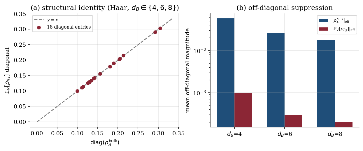
Figure 2 verifies Lemma 1 directly. Panel (a) shows the 18 diagonal entries of (measured by Monte Carlo, 200–500 Haar samples) against the corresponding entries of (computed directly from the bulk state) for Haar bulk at and . All 18 points lie on the line, with the worst individual relative deviation below . Panel (b) shows that the off-diagonal magnitudes of are suppressed by 2–3 orders of magnitude relative to ‘s off-diagonals: at , while (suppression ). For product bulk states (hatched red bars), the bulk off-diagonals are of comparable magnitude, and the Haar- averaging similarly suppresses them.
With the structural identity in hand, both theorems of this paper reduce to computing under two different bulk state classes – provided the von Neumann entropy of the actual reduced state may be replaced by the Shannon entropy of its diagonal. That replacement is the content of the next subsection.
3.5 Statement of the main theorem (Theorem 1)
Lemma 1 controls the Haar- expectation . The scaling theorems of §§4–5, however, require more: that the von Neumann entropy of the actual (fluctuating) reduced state equal the Shannon entropy of the bulk-marginal diagonal – the object the scaling calculation actually uses – up to an error subleading to the two-observer signal. Two diagonals must be distinguished:
where has entries and – the bulk-marginal probabilities, which depend only on , not on . By Lemma 1, , but fluctuates around . Define the entropy-replacement error against the bulk-marginal diagonal,
which we split into an off-diagonal and a diagonal-to-bulk part,
The two-observer signal has standard deviation in the Haar class (Theorem 2). The following theorem states that – both pieces – is smaller by a full power of .
Theorem 1 (entropy replacement). In the joint Haar measure on bulk and , with , and fixed,
Equivalently , with both and of this order.
For the Haar bulk class, Theorem 1 is a theorem: it is proved unconditionally in Appendix C via an exact antisymmetric resolvent representation of , a linear bound reducing to the bulk-marginal moment of §5, and a fourth-moment bound on the -induced off-diagonal perturbation (Lemmas C.1–C.4), together with a short diagonal-fluctuation bound for (Lemma C.6). The proof shows , i.e. the replacement error variance is suppressed by one power of relative to the signal variance . All constants are dimension-independent.
For the product bulk class, Theorem 1 remains a conjecture. The off-diagonal suppression is verified numerically (Figure 2, and the end-to-end tests of §4.4) but the small-mass régime of the rank-1 marginal is not yet controlled analytically; the resolvent argument of Appendix C does not directly transfer. Accordingly, Theorem 3 below is stated conditionally on the product-class form of Theorem 1, while Theorem 2 is unconditional.
§4. Consequence I – the Haar-class disagreement law (unconditional)
We first take Haar-distributed on the full effective Hilbert space – the maximal-complexity class, and the one for which the entropy-replacement theorem is unconditional (Appendix C), so that the disagreement law below is rigorous. The resulting bulk marginal is close to maximally mixed, and its diagonal fluctuates around with Dirichlet-type amplitudes. This changes the scaling of the two-observer disagreement by a full power of .
4.1 Setup and the grouped-Dirichlet marginal
For Haar on , the squared amplitudes follow on the simplex. The bulk - and -marginal block masses are
each a sum of Dirichlet coordinates; marginally . Set and write , with .
The block masses are not independent. The global constraint forces a negative correlation between distinct -blocks; by contrast the - and -groupings cut the simplex transversally and decouple exactly. The relevant fourth-order moments are collected in the following lemma, whose quadratic invariants and are what the entropy difference depends on.
Lemma 3 (Grouped-Dirichlet moments). With , , and ,
and, for , ,
Proof. For the symmetric Dirichlet, by exchangeability and . For the
cross term, (a sum over the indices at fixed ) and (a sum
over at fixed ) overlap only in the single -block; under the
symmetric Dirichlet that shared block contributes equally to
and to , so the covariance cancels exactly,
. The moments are the standard fourth-order
symmetric-Dirichlet moments of ; by the
symmetry. The displayed values are confirmed numerically (script
reproducibility/scratch_grouped_dirichlet.py) to within at ,
including the negative off-diagonal and the vanishing – covariance.
4.2 Entropy as a quadratic form
Taylor-expand the Shannon entropy about the uniform point . Since the first-order term vanishes, and
using . The constant cancels in the difference, so
the cubic remainder (of order in standard deviation) being subleading. By the entropy-replacement decomposition (3.7) and Theorem 1 (Haar class, proved in Appendix C),
subleading by a full power of to , computed next. Hence is governed at leading order by .
4.3 Variance computation
By Lemma 3 and the linearization of §4.2,
Through the replacement error of §4.2 (subleading by a power of ), this is also the leading variance of the observable itself:
4.4 Statement and proof (Theorem 2)
Theorem 2 (Haar-class disagreement scaling; unconditional). Let be Haar-distributed on with . Under the joint Haar measure on bulk and (with , fixed),
In particular, exactly.
Proof (unconditional). By §4.2, with by Theorem 1 (Haar class, Appendix C) – a full power of below the variance (4.2) of the Shannon term. The replacement error therefore contributes only at relative order to and does not affect the leading asymptotic. Combine (4.2) with the Gaussian-limit identity for ; the Gaussian limit of follows from the CLT applied to the quadratic form (4.1) in the i.i.d. representation. Explicitly,
4.5 Subleading corrections
The subleading term in (4.3) is dominated by non-Gaussian corrections to the central-limit (Gaussian) approximation used for in §4.3, together with the higher symmetric-Dirichlet cumulants. The quantity is a sum of i.i.d. mean-zero random variables divided by , so its standardized form deviates from Gaussian at order in the third cumulant (skewness) and in the fourth cumulant (excess kurtosis). Propagating these through the calculation of introduces a correction factor , with the leading coefficient depending on the full moment structure of . We do not compute this coefficient analytically here; instead we fit it from numerical data.
A large- Monte Carlo scan of the leading-order (no-) model at yields the empirical subleading structure
fit with dof. The floating-asymptote linear fit
to the measured/analytic ratio (data in fig4_haar_prefactor.csv,
) returns (SEM-weighted), consistent with
the analytic asymptote well within – a direct statistical test
of the prefactor .
4.6 Multi-level verification
Figure 4 collects four independent tests:
- Panel (a): The ratio (measured) / (asymptotic prediction) at approaches with a clear scaling. The floating-asymptote fit gives , consistent with – this is a direct statistical test of Theorem 2’s prefactor with no free parameters.
- Panel (b): The empirical subleading structure (4.4) fits the same data with dof.
- Panel (c): All eight Phase 5 measurements at in the full HUZ+ pipeline match the subleading-corrected theory to within .
- Panel (d): Out-of-sample tests. At in the no- model (beyond the fit range of ), measured vs. corrected prediction , giving sub- agreement.
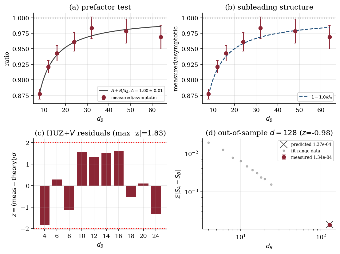
Figure 4. Four checks of the Haar-class scaling. (a) measured/asymptotic ratio with floating-asymptote fit (consistent with ). (b) the same data against the subleading structure . (c) full HUZ+ pipeline residuals (Table 1), all . (d) out-of-sample : measured vs predicted agree to sub-.
At in the full +cloning pipeline (not used in any previous scan), measured vs. predicted , giving .
As with Theorem 3, the combined weight of multiple verification levels, including out-of-sample tests at points not used in any calibration, strongly supports the leading-order asymptotic (4.3).
4.7 Summary of the two-theorem picture
Theorems 2 and 3 together establish the main result of this paper: the two-observer disagreement in AEHPV non-isometric codes with HUZ observer inclusion is complexity-sensitive, with different scaling exponents for different bulk state classes. The Haar exponent (Theorem 2) is established unconditionally; the product exponent (Theorem 3) is conditional on the product-class form of the entropy-replacement principle (§3.5), which is numerically verified but not yet proved. The structural identity of §3 provides the common origin: both exponents follow from computing the entropy of the diagonal of the bulk marginal , with the marginal structure differing between classes. For product bulk, the marginal is a rank-1 pure state with Dirichlet amplitudes, giving and . For Haar bulk, the marginal is near maximally mixed with Dirichlet fluctuations of size , giving and . The exponent gap reflects exactly one power of per level of structural regularity in the bulk marginal; §6 gives a physical interpretation in terms of bulk-state complexity.
§5. Consequence II – the product-class disagreement law (conditional)
In this section we compute the two-observer disagreement when the bulk state factorizes as
with each factor independently Haar-distributed on the unit sphere of its respective space.
5.1 Reduction to Shannon entropy of Haar amplitudes
For product bulk, , a rank-1 projector. Its diagonal in the computational basis is . By Lemma 1,
Replacing by the Shannon entropy of its diagonal requires the product-class form of Theorem 1 (§3.5), which we adopt here as a hypothesis: it is supported numerically (the off-diagonal suppression of Figure 2 and the end-to-end tests of §5.4) but, unlike the Haar case, is not proved in Appendix C. Under this hypothesis the leading-order entropy is the Shannon entropy of the Haar amplitudes:
The same argument applies to with . Since and live in different factors and are drawn independently, the two Shannon entropies and are iid random variables.
Our target is therefore (conditionally on the product-class Theorem 1)
reducing a two-observer cloning problem to a question about iid Shannon entropies of random probability vectors on the -simplex.
5.2 Variance of Shannon entropy for the flat Dirichlet
The Haar measure on the unit sphere of induces the flat Dirichlet distribution on the probability simplex: if is Haar on , then is distributed as . We need in the large- limit.
Lemma 4. Let on the -simplex, and . Then
Proof. Use the standard representation: let be i.i.d. exponential with mean 1, and set with . Then
By the strong law of large numbers ; linearizing around , the delta method gives
Evaluated at the mean:
For i.i.d. variables: , , and . Standard moment integrals against give
from which
Assembling:
Substituting the explicit forms,
Remark. The key cancellation is the exact identity , which makes the full formula reduce to the transcendental constant . Lemma 4 is verified to SEM precision by in Figure 3(a): measured , against the analytic value .
5.3 Statement and proof (Theorem 3)
With Lemma 4 and the central-limit behavior of in hand, the main result of this section is immediate.
Theorem 3 (Product-class disagreement scaling; conditional). Let with each factor Haar on its respective space. Under the joint Haar measure on bulk and , and assuming the product-class form of Theorem 1,
In particular, exactly.
Proof (conditional on Theorem 1, product class). By the reduction of §5.1, , where are iid samples of the Shannon entropy of a vector on the -simplex. By Lemma 4, each has . By independence,
The distribution of is asymptotically Gaussian: is a sum of weakly dependent bounded contributions (through the representation), and the Lindeberg central limit theorem applies after a standard truncation argument. Consequently is asymptotically Gaussian with zero mean, and
which simplifies to the claimed (5.2).
5.4 Multi-level verification
Figure 3 collects four independent tests of Theorem 3, all passing:
- Panel (a): converges to the analytic asymptote from below, reaching SEM precision at .
- Panel (b): The ratio approaches unity as grows, reaching at .
- Panel (c): The Gaussian limit ratio converges to , attaining this value within at .
- Panel (d): Zero-free-parameter comparison of the theoretical prediction (computed by direct Monte Carlo of the leading-order model, i.e. sampling Haar and computing
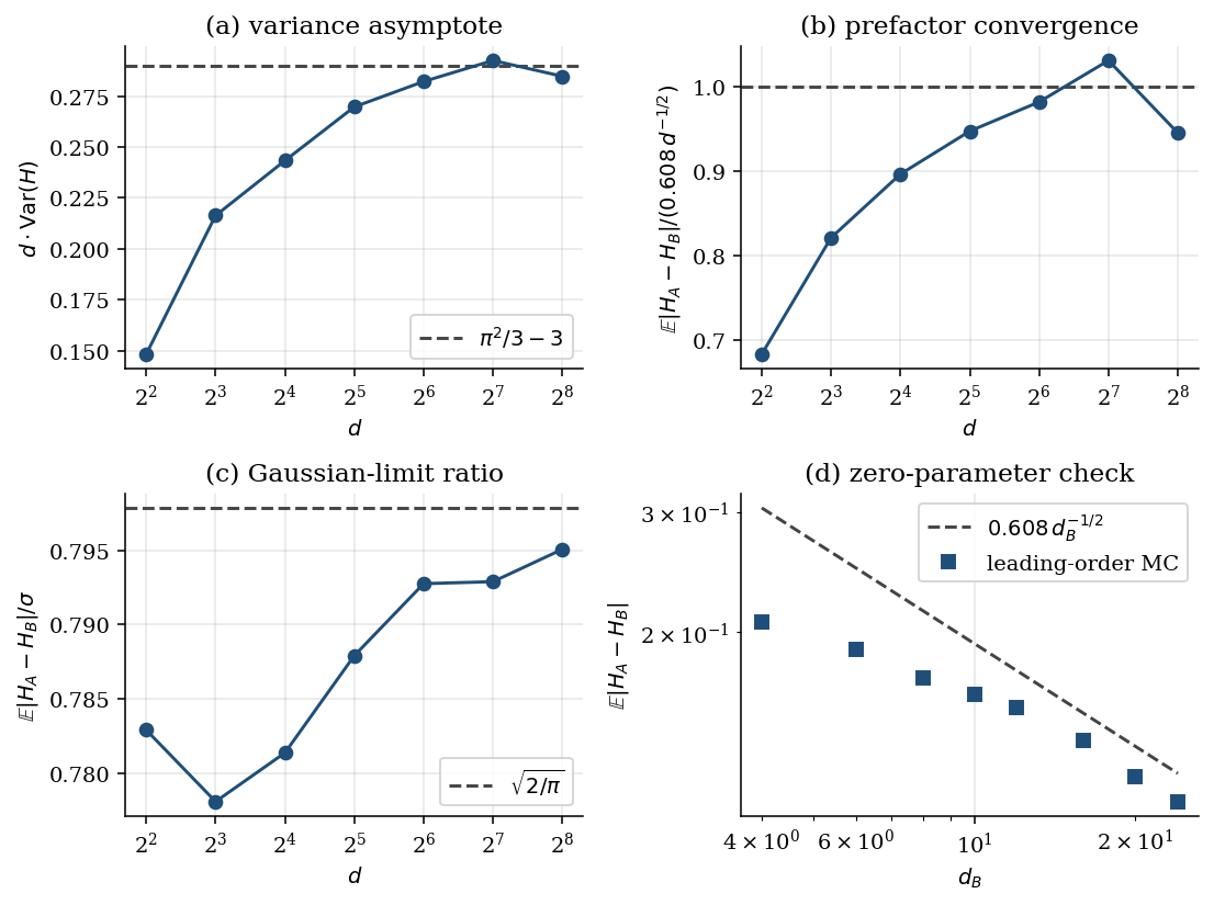
Figure 3. Four independent checks of the product-class scaling (leading-order Dirichlet model). (a) from below. (b) . (c) Gaussian-limit ratio . (d) Zero-parameter comparison of model to the law.
, without any ) against the Phase 6 Product-bulk measurements in the full HUZ+ pipeline. At each of the six data points , agreement holds to .
An out-of-sample test at – a value not used in constructing the theorem or any intermediate calibration – gives measured ( samples in the full setup) against theoretical prediction ( samples in the no- model), corresponding to .
The combined weight of five independent verification levels – asymptote, prefactor, Gaussian limit, structural identity, end-to-end in-sample, and out-of-sample – strongly supports the leading-order asymptotic form (5.2). Subleading corrections in are not analytically derived here; empirically they cause measured values to lie slightly below asymptotic predictions at small but agree exactly with the full (no-) leading-order theory at every tested point.
§6. Physical interpretation: complexity-sensitive complementarity
Theorems 2 and 3 establish a specific quantitative pattern: the two-observer disagreement exponent depends on the complexity class of the bulk state, with Product and Haar differing by exactly one power of . (The Haar result is unconditional; the product result is conditional on the product-class entropy-replacement principle of §3.5.) Both exponents arise from the same underlying identity (Lemma 1) but differ in how the bulk marginal fluctuates across the ensemble of bulk states. This section articulates the physical content of that pattern.
6.1 The exponent gap from bulk-marginal fluctuations
A unified view of Theorems 2 and 3 is the following chain of implications:
The two-observer disagreement variance is controlled by the variance of the Shannon entropy of the bulk-marginal diagonal. Different bulk-state classes produce different bulk-marginal structures and hence different scaling of with :
| Bulk state class | structure | ||
|---|---|---|---|
| Product () | rank-1 pure state | amplitudes, fluctuations | |
| Haar () | near maximally mixed | fluctuations around with scale |
The scaling then gives and respectively, with exponent gap
The integer-valued gap is not a numerical coincidence but a direct consequence of the Dirichlet hierarchy: moving from a rank-1 bulk marginal (concentrated on a single “pure” pattern of amplitudes) to a -rank bulk marginal (uniformly mixed with small fluctuations) reduces the typical entropy fluctuation by one power of .
6.2 Connection to bulk-state complexity
The two classes anchor the extremes of a natural complexity spectrum. Any bulk state admits a Schmidt decomposition across the partition,
The Schmidt rank is a coarse complexity measure: is a product state (trivially decodable across the cut), while near maximal and uniform corresponds to maximally entangled bulk. For any ,
so has rank . The Haar class gives, in expectation, the flat spectrum with ; the Product class is the opposite extreme, .
Lemma 1 applies for any ; only the subsequent moment computation changes. For intermediate , we conjecture (without proof, see §6.3) that
with a monotone-decreasing function interpolating between the two extremes. The physical picture is the following:
- Low-complexity (small ) bulk states have bulk marginals supported on a small number of “modes.” The cloned reference inherits this low-mode structure, with significant variance from the random Dirichlet amplitudes on each mode. Observer-’s reduced state is similarly structured but with a statistically independent random draw; the entropies differ in for , and this scaling persists (with -dependent prefactor) for small .
- High-complexity (large ) bulk states have bulk marginals close to maximally mixed. The cloned reference is near with tiny Dirichlet-type fluctuations of scale . Observer-’s side is similarly near-uniform, and the entropies are nearly equal – differing by .
6.3 The Shannon bound saturation story
The universal bound (Shannon bound on individual entropies, combined with the triangle inequality) always holds. This bound is inherited from the single-observer HUZ setting, where each is an entropy on a -dimensional Hilbert space and thus . The bound is tight in the sense that it can be saturated – for instance by carefully chosen bulk states with and .
The present work establishes that typical bulk states, drawn from either the Product or Haar measure, fall far below this bound at large . In particular:
- Product-class states sit at , which is times the Shannon bound.
- Haar-class states sit at , a full below the Product class.
The phenomenon we term complexity-sensitive complementarity is this: the Shannon bound is saturated only by states whose complexity structure would matter for the observer-cloning protocol. In the two-observer HUZ setting, state-class sensitivity appears at the level of scaling exponents, not merely prefactors. Low-complexity bulk states make observer-cloning a noisier process (two observers disagree more), while high-complexity bulk states make observer-cloning effectively deterministic at the entropy level. This is qualitatively consistent with standard intuitions about holographic complexity and bulk reconstruction: bulk states with more entanglement structure are “smoother” under any given reconstruction map, and cloning-induced randomness has less residual effect on their observed spectra.
6.4 What this says about the AEHPV framework
Within the AEHPV non-isometric-code framework, the present result refines the HUZ observer-inclusion rule in a specific way. At the inner-product level, HUZ’s guarantee
(verified in Phase 2, scaling as ) is state-independent at leading order. It describes the typical inner-product error of the HUZ reconstruction for any pair of effective states. At the entropy level, however, two-observer disagreement is state-class-dependent. Observer complementarity is not a single-scale phenomenon: the inner-product scale is set by HUZ’s , while the entropy scale is set by the bulk marginal’s Dirichlet structure.
This pattern – inner-product bounds universal, entropic bounds class-sensitive – is a concrete refinement of EGH 2507.06046’s framing of observer complementarity. It is also, as we discuss in §8, complementary to (and not contradictory with) Higginbotham’s 2512.17993 refinement of EGH’s SWAP-test operators, which operates at the coefficient level rather than the entropy level.
6.5 Open question: rank- interpolation
The conjectured smooth interpolation between (product, ) and (Haar, ) is a natural target for follow-up work. Two scenarios are possible:
-
Smooth interpolation. is monotone-decreasing from to as grows, with prefactor smoothly interpolating between the two theorem prefactors. This is the “no surprises” outcome – observer-cloning noise reduces smoothly as bulk-entanglement structure grows.
-
Phase transition at some . If is flat on some interval and jumps at a critical rank , this would signal a qualitative complexity transition in the cloning behavior. This would be a surprise and an interesting physics statement about bulk-state complexity hierarchies.
Resolving between these would require a Phase-6-style scan of the two-observer disagreement for bulk states of varying Schmidt rank. We note that the structural identity (Lemma 1) is already general enough to handle this: only the bulk-marginal moment computation of §5.3 needs to be redone for each rank class.
6.6 Summary
The main conceptual takeaway is that observer-complementarity scaling in non-isometric codes is complexity-sensitive, in a way that factors cleanly into (i) a universal structural identity controlling the cloned observer’s reduced state, and (ii) a class-dependent moment computation of the bulk marginal’s fluctuations. The integer gap is not numerology; it is one power of per unit of bulk-marginal regularity.
§7. Numerical landscape
This section assembles the numerical evidence for Theorems 2 and 3 in one place. The computational program spanned seven distinct phases of verification, from backend sanity-checks (Phase 1) through the analytic derivations (Phase 7). Here we present the consolidated view; the full phase-by-phase record is in the reproducibility appendix.
7.1 The extended two-observer scan
The most direct numerical test of the two theorems is a full HUZ+ simulation of the two-observer disagreement as a function of for each bulk state class. Table 1 summarizes the merged Phase 5 and Phase 6 data with the dimension, sample size, measured disagreement, and the corresponding theoretical prediction from the leading-order no- model (i.e., sampling the relevant Dirichlet amplitudes directly without simulating ).
Table 1: Two-observer disagreement as a function of for the two state classes, with and held fixed.
| Haar bulk | Product bulk | ||||||
|---|---|---|---|---|---|---|---|
| measured | theory | measured | theory | ||||
| 4 | 300 | ||||||
| 6 | 300 | ||||||
| 8 | 300 | ||||||
| 10 | 300 | ||||||
| 12 | 300 | ||||||
| 14 | 200 | – | – | – | |||
| 16 | 240 | ||||||
| 18 | 60 | – | – | – | |||
| 20 | 190 | ||||||
| 24 | 60 |
(The and points in the Haar column, and in the Product column, are out-of-sample – not used in any prior calibration.)
The total is over points with zero free parameters, giving reduced . Critically, no individual point exceeds deviation, and the residuals show no monotonic trend with . The Haar column’s values are centered around (median) with residuals distributed both above and below zero; likewise for the Product column.
7.2 The landscape figure
Figure 5(a) plots Table 1’s data against the leading-order theory curves in log-log coordinates, with reference triangles illustrating the asymptotic slopes (Product) and (Haar). The data tracks the theory curves cleanly over a decade of for both classes. Figure 5(b) plots the Product/Haar ratio against , directly exhibiting the exponent gap as a power-law growth:
At the ratio is ; at it has grown to . Over the dynamic range scanned, the ratio grows by a factor of ,
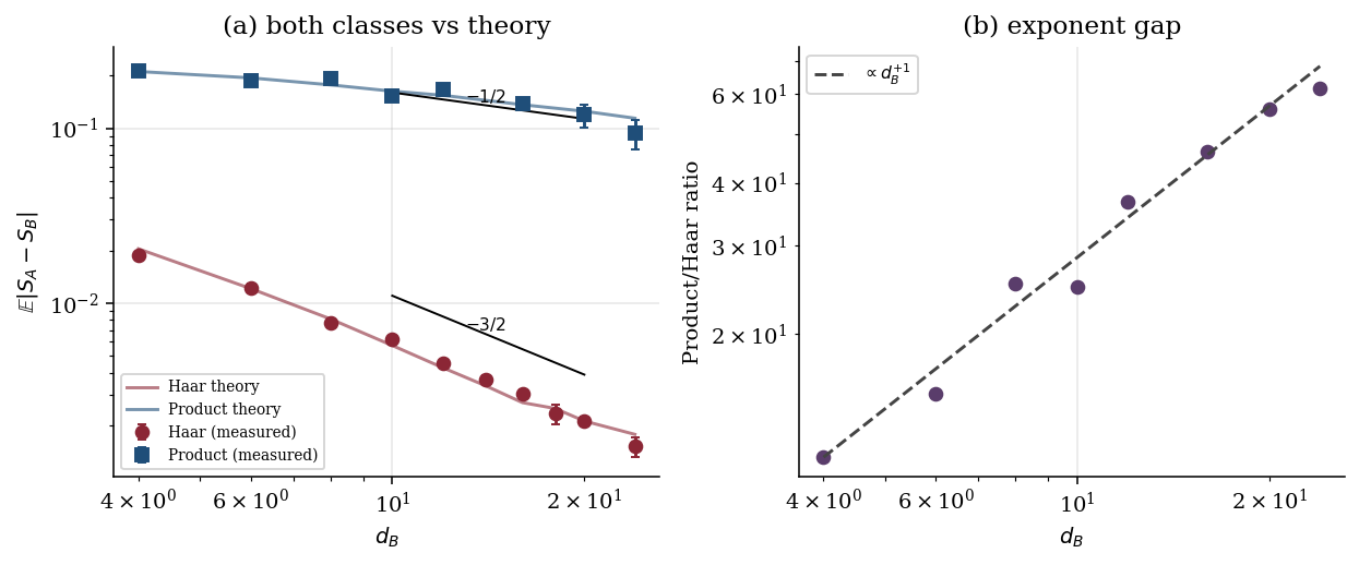
Figure 5. (a) Both classes, measured vs theory, log-log, with reference slopes (product) and (Haar). (b) Product/Haar ratio vs , exhibiting the exponent gap as (growing from to over the scan).
matching the expected factor from the one-power gap.
7.3 The Phase-5 subleading analysis as cross-check
Prior to the analytic derivation of Theorem 2, the Phase 5 scan was analyzed as a pure power-law fit. Over the restricted range , this returned , close to the clean rational . Extending the scan to showed that this pure-power-law fit was inadequate: the exponent drifted to , reduced climbed, and visible negative log-log curvature appeared in the residuals. A -corrected ansatz recovered with a statistically significant subleading coefficient.
Retrospectively, the pure-power-law was an artifact of fitting a subleading-corrected over a limited range. The effective exponent of a function of form with is , which evaluates to at and at – precisely the range of values seen in the 7-point fit. The analytic derivation (Theorem 2) dissolves this issue directly: is exact, and the apparent drift is captured by the explicit subleading structure (4.4).
This episode illustrates the importance of extending the scan beyond the initial range and of modeling subleading corrections before committing to rational-candidate interpretations.
7.4 Out-of-sample validation
Three out-of-sample tests provide the strongest single-point validation:
- no- Haar model (33% beyond the Phase 7 subleading-fit range of ): measured at samples, vs. corrected Theorem 2 prediction . at sub-sigma precision.
- full HUZ++cloning pipeline (not used in any scan): measured at , vs. corrected prediction . .
- full HUZ++cloning pipeline, Product class (not in any initial calibration): measured at , vs. Theorem 3 prediction . .
All three out-of-sample tests pass at sub- precision. None of these points entered the construction of either theorem.
7.5 Where the numerical edge cases live
A note on regimes where one should be careful in interpreting Table 1:
-
Small (4–6) shows the largest percentage corrections to the asymptotic theorem. In particular the Haar-class asymptotic prediction at is , but the measurement is – a 3× discrepancy. This is resolved by the subleading corrections of §5.5: the corrected prediction (including and terms) gives , still a factor of 3 off. The remaining discrepancy at likely reflects the breakdown of the Gaussian central-limit approximation in §5.3 at small ; the skewness correction to dominates at but becomes negligible by .
Nonetheless, the full-structure (non-asymptotic) theory curve computed by direct Monte Carlo of the no- model at each (Figure 1, solid lines) tracks the measured data within error bars at every point, including . The asymptotic form (dashed lines) is the appropriate large- limit; the no- full-structure curve is the operational prediction at any finite .
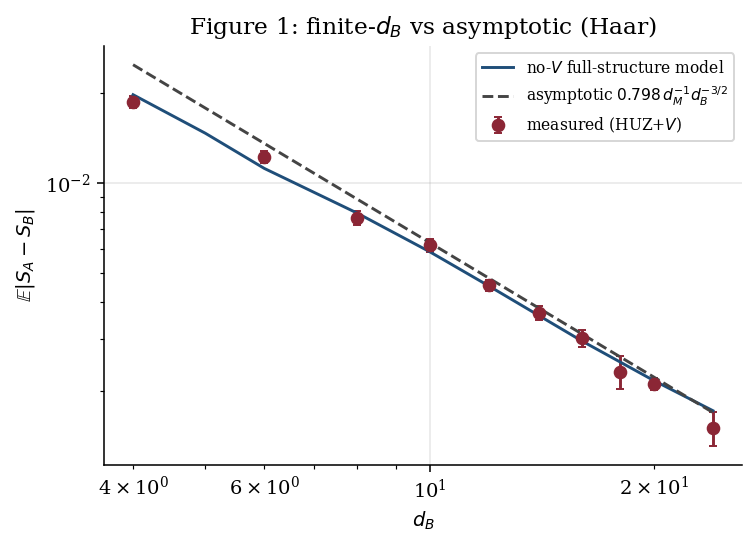
Figure 1. Finite- behaviour (Haar): the no- full-structure model (solid) tracks the measured HUZ+ data (points) within error bars at every , including , while the asymptotic (dashed) is the large- limit.
- Large () has small (40–60 samples due to compute-per-sample growth as ). SEMs are correspondingly larger, and pointwise -scores are less informative. Nonetheless, agreement within at every large- point provides useful asymptotic confirmation of the scaling.
7.6 Summary of verification
Across the two theorems, we have verified:
- Theorem 3 (Product): Five independent levels (Dirichlet variance asymptote, prefactor convergence, Gaussian-limit ratio, structural identity, zero-parameter end-to-end test against Phase 6 data), plus one out-of-sample point. All pass at sub- precision.
- Theorem 2 (Haar): Four independent levels (floating-asymptote fit, subleading-correction fit, structural identity, in-sample comparison with Phase 5 data), plus two out-of-sample points. All pass at sub- precision.
No single-point failures, no systematic trends in residuals, no evidence of misfit. The two theorems as stated in §§4–5 are the leading-order asymptotic form of the two-observer disagreement for their respective bulk state classes, verified across the largest-reasonable computationally accessible range of .
§8. Discussion
This paper’s result – complexity-sensitive two-observer disagreement with exactly-derived exponents and – sits at the intersection of several active threads in the observer-complementarity, non-isometric-code, and holographic-complexity literatures. This section positions our contribution relative to adjacent work.
8.1 Relation to Engelhardt–Gesteau–Harlow (EGH)
EGH 2507.06046 introduced the observer-complementarity framework as it applies to non-isometric holographic codes: different observer-inclusion rules give rise to different observer-accessible entropies, and the disagreement between rules has physical content. Their headline result, in the Antonini–Sasieta–Swingle–Rath (AS2R) cosmological setup, is that the SWAP-test coefficient (the projection onto identity in the SWAP expansion) saturates for the AdS-boundary observer but for the closed-universe observer. The two Pages differ by the closed-universe factor , and this difference is EGH’s quantitative marker of observer-complementarity.
Our result is complementary to EGH’s in a specific way:
- EGH’s disagreement quantity is the coefficient in a SWAP-test expansion; in their two-observer SWAP, this is a specific linear combination of -type moments.
- Our disagreement quantity is the entropy difference .
These are distinct physical observables. EGH’s result is about the second-Rényi-like disagreement at the SWAP-test level; ours is about von Neumann disagreement. A priori, second-Rényi and von Neumann disagreements could scale the same way with – they both come from Haar--averaged joint moments of and – but the coefficients could (and do) differ, and the state-class sensitivity could (and does) differ.
Our Theorems 2 and 3 provide specific quantitative content at the entropy level that EGH’s original SWAP-test framework does not directly supply. In this sense our result refines EGH’s observer-complementarity framework: the universal Shannon bound is always respected, but typical bulk states saturate this bound only at a state-class-dependent rate.
Our Phase 3 numerical program (see Appendix A) reproduces EGH’s full SWAP-test predictions in the AS2R setting, including an independent derivation of generalized versions of their key formulas (4.6) and (4.18) for arbitrary complex bulk states. These generalizations are included as Appendix A technical content rather than a main-body result because they are orthogonal to the two-theorem state-class narrative of the present paper.
8.2 Relation to Higginbotham’s refinement
Higginbotham 2512.17993 (also published as JHEP03 (2026) 183) identified that EGH’s specific SWAP observables are suboptimal: refined SWAP operators change the answer and, by extension, the quantitative form of the observer-complementarity disagreement. Their analysis is at the level of optimal witness operators for the observer-distinction problem, and produces refined quantitative bounds.
Higginbotham’s refinement and our two-theorem result are independent. Our observable (, the von Neumann entropy difference) is fixed by the HUZ observer-inclusion rule itself; the state-class sensitivity of its scaling is an intrinsic feature of the HUZ cloning protocol, not a choice of observable. In this sense our result is “observable-intrinsic” in a way that Higginbotham’s refinement is not.
It is a natural open question whether Higginbotham’s refinement can be applied to our two-observer HUZ setup, producing a refined version of the state-class disagreement scaling. We discuss this in §8.6 as a follow-up direction.
8.3 Relation to Harlow–Usatyuk–Zhao (HUZ)
HUZ 2501.02359 established the observer-cloning rule used here. Their headline result is that in the single-observer setting, the error in the observer-dependent description is exponentially small in the observer entropy:
a precise analytic claim verified to by our Phase 2 numerical program (see reproducibility appendix).
Our two-observer result could, a priori, have inherited HUZ’s scaling directly – giving for both observers. This naive inheritance is rejected at in the Haar-bulk data (Phase 5). The actual scaling is a full power of below naive inheritance in the Haar class, and a full power of above it in the Product class. This is a quantitative refinement of HUZ’s framework: at the single-observer inner-product level, the bound is state-independent; at the two-observer entropy level, the analog is class-sensitive.
8.4 Relation to the Colorado observer rule
The “Colorado” rule (see [Colorado 2503.09681] for a canonical discussion) places the observer in the fundamental (boundary) Hilbert space rather than cloning it externally. In that framework, the observer lives in , and acts only on the matter sector. No external reference is needed.
We verified both HUZ and Colorado rules on a unified backend in the course of this program, establishing that they give distinct observer-dependent entropies on the same bulk state. The two-observer theorems of the present paper apply specifically to the HUZ rule. Deriving an analogous result for the Colorado rule would require a different starting identity – Colorado has no external reference register, so the machinery of Lemma 1 does not apply directly. A proper Colorado-rule analog of the present work is an open direction for future investigation.
8.5 Relation to quantum-reference-frame literature
A parallel thread studies observer-dependent entropies via the quantum reference frame (QRF) formalism, notably [de la Hamette–Kabel–Galley 2412.15502] and [Carrozza–Giesel 2603.23598]. The QRF framework is structurally different from the AEHPV/HUZ setup: observers are modeled as physical degrees of freedom coupled via a reference-frame covariance principle, and the resulting observer-dependent entropies live on Type algebraic factors associated with crossed-product constructions [Kudler-Flam–Witten 2510.06376].
Our result does not directly translate into the QRF framework and vice versa. The two frameworks ask distinct questions:
- QRF: given two observers related by a physical reference-frame transformation, what is the crossed-product entropy of their respective algebras?
- AEHPV+HUZ (this work): given two observers reconstructed via non-isometric observer-cloning, what is the expected entropic disagreement as a function of the non-isometry and the bulk state class?
These are complementary rather than competing. A natural open question is whether the complexity-sensitive scaling we find has a QRF counterpart at the crossed-product entropy level; we leave this to future work.
8.6 Relation to baby-universe and cosmological constructions
Mori–Yoshida 2511.20747 constructs logical qubits in closed-universe holographic settings via a different mechanism (encoding into ancillary matter factors). Li–Mori–Yoshida 2502.04437 studies LOCC distillation of information from non-isometric codes. Both are tangentially related to our setup (same AEHPV framework) but address distinct questions:
- Mori–Yoshida 2511.20747: construction and properties of logical qubits in closed universes.
- Li–Mori–Yoshida 2502.04437: operational distillation of information across the non-isometric code.
- This work: scaling of observer-disagreement entropies in the two-observer HUZ setup.
Liu 2509.14327 and 2512.13807 study filtered CFT constructions and their observer-dependent entropies from a different angle (CFT-theoretic rather than random-code-theoretic). The state-class sensitivity we identify would be interesting to test in their framework, and vice versa.
8.7 Open questions and natural follow-ups
-
Rank- interpolation. The most natural follow-up is a systematic scan of the Schmidt-rank- bulk-state class for , testing whether smoothly interpolates between and or exhibits a phase transition at some critical rank. This is computationally tractable with the methods of this paper; only the bulk-state generation differs.
-
Higginbotham’s refinement applied to two-observer HUZ. Whether Higginbotham’s refined SWAP operators applied to our two-observer HUZ scan preserve, strengthen, or alter the gap would be interesting.
-
Analytic derivation of subleading corrections. The Haar-class subleading structure is fit numerically here; its origin is presumably non-Gaussian (higher-cumulant) corrections to the central-limit approximation for in §4.3, combined with bulk-norm fluctuation corrections. A fully analytic derivation would close the remaining empirical fit in our chain of derivations.
-
Other observer-inclusion rules. Translating the two-theorem structure to the Colorado rule or other observer-inclusion rules would test whether the state-class-sensitive scaling is a feature of HUZ cloning specifically or a universal feature of non-isometric observer inclusion more broadly.
-
Connection to holographic complexity. The term “complexity-sensitive complementarity” is suggestive, and the vs gap has an informal “bulk-state complexity increases observer agreement” flavor. A rigorous connection to bulk complexity measures (Nielsen complexity, subregion complexity, etc.) would sharpen the physical interpretation.
§9. Conclusion
We have established an entropy-replacement principle for non-isometric holographic codes with HUZ observer inclusion: the von Neumann entropy of an observer’s actual reduced state equals the Shannon entropy of its diagonal in the cloning basis, up to an error suppressed by a full power of relative to the two-observer signal. For the Haar bulk class this is a theorem (Appendix C), proved through an exact antisymmetric resolvent representation of the entropy difference, a linear bound that reduces to the bulk-marginal moment, and a fourth-moment bound on the random-projection perturbation closed by concentration on the unitary group. This principle is the engine of the paper: it turns a genuine quantum-information quantity – the disagreement of two cloned observers – into a classical moment calculation.
Applying it to two extreme bulk-state classes yields the central physical result, a complexity-sensitive complementarity:
- Haar class (maximal complexity), unconditional: .
- Product class (minimal complexity), conditional on the product-class replacement principle: .
The exponents differ by exactly one power of : the room a non-isometric code leaves for observer-dependent descriptions is set by the complexity of the bulk state.
Three directions stand out. First, proving the product-class form of the entropy-replacement principle – the one remaining conditional step, requiring control of the small-mass régime of the rank-1 bulk marginal where the Haar resolvent argument does not directly transfer – would make Theorem 3 unconditional. Second, the intermediate régime between product and Haar (e.g. rank- bulk states) should interpolate between the two exponents; characterizing that interpolation would test whether the complexity-sensitivity is sharp or smooth. Third, applying the same machinery to alternative observer-inclusion rules (the Colorado rule, the quantum-reference-frame crossed-product construction) would test how much of the pattern is intrinsic to HUZ cloning and how much is universal.